The normal distribution

Normal distribution, also known as the Gaussian distribution, is a probability distribution that is symmetric about the mean, showing that data near the mean are more frequent in occurrence than data far from the mean.

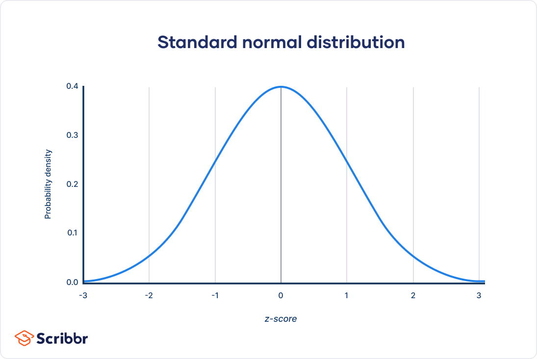
Normal distribution characteristics:

1. Symmetrical

2. Area = 1

3. Probability never hits 0

4. Describe by mean and standard deviation

Distribution of Amir's sales

#1
# Histogram of amount with 10 bins and show plot
amir_deals['amount'].hist(bins=10)
plt.show()

Probabilities from the normal distribution

#1
# Probability of deal < 7500
prob_less_7500 = norm.cdf(7500, 5000, 2000)

print(prob_less_7500)

#2
# Probability of deal > 1000
prob_over_1000 = 1 - norm.cdf(1000, 5000, 2000)

print(prob_over_1000)

#3
# Probability of deal between 3000 and 7000
prob_3000_to_7000 = norm.cdf(7000, 5000, 2000) - norm.cdf(3000, 5000, 2000)

print(prob_3000_to_7000)

#4
# Calculate amount that 25% of deals will be less than
pct_25 = norm.ppf(0.25, 5000, 2000)

print(pct_25)

Simulating sales under new market conditions

# Calculate new average amount
new_mean = 1.2 * 5000

# Calculate new standard deviation
new_sd = 1.3 * 2000

# Simulate 36 new sales
new_sales = norm.rvs(new_mean, new_sd, size=36)

# Create histogram and show
plt.hist(new_sales)
plt.show()

The central limit theorem

The sampling distribution of statistics becomes closer to the normal distribution as the number of trials increases.

Rolling the dice 5 times

dice = pd.Series([1, 2, 3, 4, 5, 6])

# Roll 5 times
# 1st attempt
samp_5 = dice.sample(5, replace=True) 
np.mean(samp_5) # Out: 2

# 2nd attempt
samp_5 = dice.sample(5, replace=True) 
np.mean(samp_5) # Out: 4.4

# 3rd attempt
samp_5 = dice.sample(5, replace=True) 
np.mean(samp_5) # Out: 3.8

The CLT

# 1.
# Create a histogram of num_users and show
amir_deals['num_users'].hist()
plt.show()

# 2.
# Set seed to 104
np.random.seed(104)

# Sample 20 num_users with replacement from amir_deals
samp_20 = amir_deals['num_users'].sample(20, replace=True)

# Take mean of samp_20
print(np.mean(samp_20))

# 3 
sample_means = []
# Loop 100 times
for i in range(100):
  # Take sample of 20 num_users
  samp_20 = amir_deals['num_users'].sample(20, replace=True)
  # Calculate mean of samp_20
  samp_20_mean = np.mean(samp_20)
  # Append samp_20_mean to sample_means
  sample_means.append(samp_20_mean)

print(sample_means)

# 4
# Convert to Series and plot histogram
sample_means_series = pd.Series(sample_means)
sample_means_series.hist()
# Show plot
plt.show()

The mean of the means

# Set seed to 321
np.random.seed(321)

sample_means = []
# Loop 30 times to take 30 means
for i in range(30):
  # Take sample of size 20 from num_users col of all_deals with replacement
  cur_sample = all_deals['num_users'].sample(20, replace=True)
  # Take mean of cur_sample
  cur_mean = np.mean(cur_sample)
  # Append cur_mean to sample_means
  sample_means.append(cur_mean)

# Print mean of sample_means
print(np.mean(sample_means))

# Print mean of num_users in amir_deals
print(np.mean(amir_deals['num_users']))

The Poisson Distribution

Poisson process

• Events appear to happen at a certain rate, but completely at random.

• Time unit is irrelevant, as long as we use the same unit when talking about the same situation.

• Examples:

  • Number of animals adopted from an animal shelter per week

  • Number of people arriving at a station per hour

  • Number of earthquakes in Indonesia per year

Poisson distribution

• Probability of some # of events occurring over a fixed period of time

• Examples:

  • Probability of > 6 animals adopted from an animal shelter per week

  • Probability of 11 people arriving at a station per hour

  • Probability of < 9 earthquakes in Indonesia per year

• Describe by a value called lambda (λ) is an average number of events per time interval

• Lambda is the distribution's peak

• The CLT still apllies

from scipy.stats import poisson
poisson.pdf(5, 8) # P(8 adoptions per 5 week)
poisson.cdf(5, 8) # P(8 adoptions in a week <= 5)
1 - poisson.cdf(5, 8) # P(8 adoptions in a week > 5)
poisson.rvs(8, size = 10) # Sampling from poisson distribution

Tracking lead responses

# Import poisson from scipy.stats
from scipy.stats import poisson

#1
# Probability of 5 responses
prob_5 = poisson.pmf(5, 4)

print(prob_5)

#2
# Probability of 5 responses
prob_coworker = poisson.pmf(5, 5.5)

print(prob_coworker)

#3
# Probability of 2 or fewer responses
prob_2_or_less = poisson.cdf(2, 4)

print(prob_2_or_less)

#4
# Probability of > 10 responses
prob_over_10 = 1 - poisson.cdf(10, 4)

print(prob_over_10)

More probability distributions

Modelling time between leads

#1
# Import expon from scipy.stats
from scipy.stats import expon

# Print probability response takes < 1 hour
print(expon.cdf(1, scale=2.5))

#2
# Print probability response takes > 4 hours
print(1- expon.cdf(4, scale=2.5))

#3 
# Print probability response takes 3-4 hours
print(expon.cdf(4, scale=2.5) - expon.cdf(3, scale=2.5))